The Hyperscience Machine Learning Engineers decided to challenge our current table algorithms with a graph neural networks (also known as GraphNNs) approach based on recently published papers in the field.
We won’t be aiming to encompass the entire generality of GraphNNs within this blog post. Rather, our objective is to showcase a potential solution to a problem. If you’re interested in the variety of tools you can use with GraphNNs, please refer to this paper.
The below exposition is based on two recent papers: Reba, et al. and Qasim, et al. Throughout the piece, we’ll explain how table concepts can be translated into graphical concepts, and how graphs can be transformed into trainable Neural Networks.
Ultimately, although the GraphNNs didn’t outperform our current solution, our team liked the natural mapping between table and graph concepts.
Introduction to Tables
Much of the data in documents is organized into tables. At Hyperscience, we want to unlock this data for our customers. People often associate tables with a grid, as seen below.

A simple table with three records and columns that span from top to bottom.
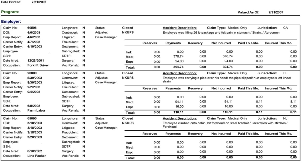
However, as we started exploring the versatility of tables, we determined that their various applications do not conform to the traditional definition of a spreadsheet. For example, although the following image displays three records, there is no clear header.

No clear definition of columns from top to bottom.
We faced another challenge when examining tables. Typically, documents containing tables are formatted with Excel — making the entire document a table by default. However, it’s sensible to assume people would treat different parts of the document as multiple tables depending on their data needs.

Although this entire document is technically a table, only the circled table is relevant.
This example brought us to the conclusion that in order to extract relevant information for our clients, it is not enough to simply be aware of a table structure. We must also understand the meaning of its contents.
Modeling Tables
Review of Current Research
To summarize the challenges observed in the previous section:
- Tables do not always follow a streamlined structure.
- Semantic understanding is required to define rows and columns in a table.
This prompted us to look for a solution that is flexible enough to meet these challenges. Graph neural networks seemed like a good resolution.
Table Structure
Prior to starting with the Machine Learning (ML) models, let’s define the structures of a table.
- A cell is a section of the table that cannot be further split.
- A column is a collection of cells that have the same semantic meaning. An example of this is the total per line item in an invoice. Columns don’t need to be vertically aligned.
- A row is a collection of cells that belong to the same record. It is possible that a row has subrows within it.

Turning a Table into a Graph
A graph consists of edges and vertices.

For example, the vertices of the above image are are V = {1, 2, 3, 4, 5, 6} and the edges are E = {{1, 2}, {1, 5}, {2, 3}, {2, 5}, {3, 4}, {3, 5}, {4, 6}}. Let us denote the number of vertices in the graph with N. For our example, N=6. Traditionally, a graph may be directed (the order of vertices in an edge matters), or undirected (the vertices in an edge do not have an order). In this example, and for the remainder of this blog post, we will focus on undirected graphs.
How can we translate graphical concepts of edges and vertices into a table’s defining characteristics of cells, rows and columns? Following the insights within this paper, we are going to define three graphs: one for cells, one for rows, and one for columns. Let’s look at a table after optical character recognition (OCR).

As you can see, the OCR outputs segments which consist of two major details:
- The bounding boxes around each word.
- The text within the bounding box, known as the transcription.
Let’s first construct the column graph. Let’s give numbers to the segments from the OCR and define them as vertices.

The green numbers represent the number of the vertex. There are N=24 vertices in this example.
Next, we define the edges. We are going to put an edge between two segments if they belong to the same column. Let’s put the edges that correspond to the column “Shift.”
The vertices for the column “Shift”.
The associated edges are: {6, 12}, {12, 18} and {6, 18}. The last edge is not clearly visible due to an overlap.
After adding the other column, the complete column graph looks like this:

The column graph. Some edges are not clearly visible due to an overlap.
The graph for rows will look like this:

The row graph. Some edges, such as {18, 23}, are not clearly visible due to an overlap.
For the cell graph, the segment number 6 – “A” will be connected only to itself, i.e. there will be an edge {6, 6}. The cell “8 hours” consists of two segments: 7 and 8. Hence, it will have edges {7, 7}, {7, 8} and {8, 8}.
The row and column graphs will also have an edge that connects to the same vertex for each vertex in the table. The edge is not visualised above in order to reduce the clutter.
Turning a Graph into a Neural Network
In the previous section, we turned an annotated table into three graphs which represent the ground truth for the table. In this section, we are going to construct a graph for a document without ground truth. This graph will be the basis from which we are going to infer the cell/row/column ground truth graphs in the next section. This base graph will again have segments at its vertices. Before looking into how we can define the edges, let’s understand how we can add features to the vertices.
Vertex Features
For each vertex i=1,…N, we will attach a vector real numbers vi ∈ R#vertex feature. The vertex features are derived from the content of the segment. In particular, we concatenate the following:
- A word embedding as described in our previous blog post.
- Positional embedding also described in our previous blog post.
- The features of the center of the segment from a shallow CNN.
Connectivity
The obvious choice would be to create a fully connected graph by placing an edge between every two segments. This will produce N(N-1)/2 edges, which can get unmanageable for documents with a few thousand words. To reduce the computational complexity, we can choose between two strategies.
The first approach is to connect segments which are aligned vertically or horizontally, as used by Riba, et al.

Source: Riba, et. al.[https://priba.github.io/assets/publi/conf/2019_ICDAR_PRiba.pdf]
As seen on the above image, most vertices are typically connected to two or three related segments.
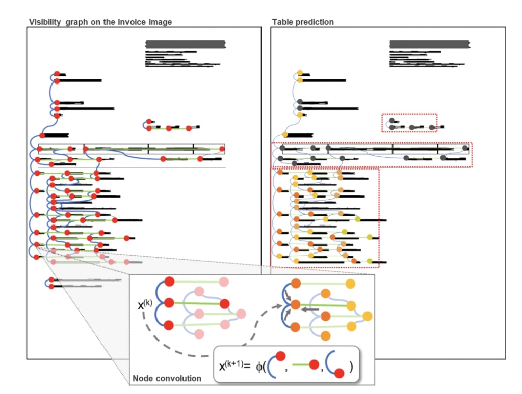
Alternatively, we can connect each node to its k-nearest neighbors as used by Qasim, et. al. We’ve seen that connecting geometrically aligned segments carries more information than connecting them based on physical distance.
In either case, we significantly reduce the computational cost from O(N^2) to O(kN) in the subsequent calculations.
Edge Convolutions
We have successfully created our base graph and we attached a vector of features vi to each vertex, but we haven’t shown how to make calculations with them. In the paper Dynamic Graph CNN for Learning on Point Clouds, the idea for a convolution on an image was extended to a graph. A PyTorch implementation of Edge Convolutions as defined there can be found here. Unlike image convolutions, which change the dimension of the image, edge convolutions keep the dimension of the vertex features. Let’s explore the formula for edge convolutions in detail:

vi are the features of vertex i before the convolution and vi’ will be the features after the convolution. N(i) is the set of all neighbouring verecies (i.e. connected by an edge) to i. vj–vi represent “relative” features. They are relative because after subtracting vi, only the relative difference between i and its neighbour j remains. We concatenate the features of the vertex vi with the relative features to its neighbor j, which we denote by vi||vj–vi. Then, we apply a neural network hΘ to this vector. Finally, we aggregate the result for each neighbouring vertex by taking the sum. We can swap the sum with other aggregating functions, such as the mean or the max.
After applying the convolution the new vertex features vi’, we’ll have information not only about them, but also about their immediate neighbours. If we apply a second edge convolution to the transformed features v’, we’ll get information about vertices which are two edges apart. Just like doing several convolutions in a sequence gives a bigger receptive field, using edge convolutions in sequence makes it possible to use information from edges that are not immediately adjacent. In practice, between three and five edge convolutional layers are used. Using several convolutions will ensure that some information can be exchanged with each vertex even if the graph is not fully connected. We aim to choose the number of convolutional layers, K, in such a way that on average, two edges are at most K apart from each other.
Predicting a Table with a Graph
The base graph can be used as a shared source of interaction between the segments for the prediction of the three ground truth graphs following Qasim, et. al. Let’s first understand how we can identify a single cell from all the segments in the document. Recall that the ground truth graph for cells has an edge between two segments if they belong to the same cell. Thus, the classification task we want to solve is: given two segments, do they belong to the same cell?
In order to achieve this, we feed the features of two segments from the base graph after the edge convolutions to a Dense Feedforward Network. Similarly, we have dense nets for rows or columns. As we have to do classification for each pair of segments, this will bring us back to O(N^2) territory. In order to make training feasible, we sample m pairs during training and calculate the loss only for them.

Source: Qasim, et. al. https://arxiv.org/pdf/1905.13391.pdf
At inference, speed is not critical, so we run all pairs of segments through the three dense layers for each predicted document.
Training Details
The output of the Dense Nets for cells are treated as logits for the binary classification task: these two segments are part of one cell. Similarly, the dense nets for rows and columns produce logits for a shared row or column, respectively. We compute the mean of the softmax cross entropy for each pair of segments which were sampled for the task. Finally, we sum the losses of the cell, row, and columns with predefined weights and backpropagate with a standard Adam optimizer.
Results
To measure the performance of our models, we adopted two metrics:
- Cell accuracy
- How many cells we classified as correct out of all cells in the test set.
- Straight-through processing
- What portion of the documents in the test set are predicted perfectly.
On our test dataset we achieved 84% cell accuracy and 7% straight-through processing. This is subpar to our current models but still shows some potential.
Author’s Note: Thanks to Lili Slavkova and Iliya Zhechev for their work on the experiment. Also, thanks to Ivo Strandjev and Kris Tashkov for their article review.

